Noises often degrade images. Noise can occur during image capture, transmission, etc. Noise removal is an essential task in image processing. In general, the results of the noise removal have a strong influence on the quality of the image processing techniques. Today in this post, I’ll be sharing an intuitive approach to noise reduction. I’ll be referring to this paper and this post to maintain the standard flow.

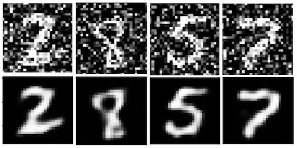
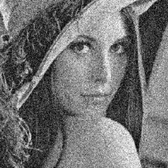
We will be trying to transform the noisy image, as shown in the top half of the image below, to one that looks close to the bottom half. This will be covered over multiple posts. In this post we will talk mainly about Moving Average Filters or MAFs. We can observe that at many places in this black and white image, there is an occurrence of an undesirable black pixel in place of white and vice-versa. We call it Salt and Pepper noise, Obviously!

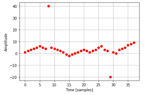
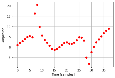
Let’s start with the one-dimensional case. Firstly, Let’s generate a discrete impulse train with the python code given below. I’ve included two noise-like points of 40 and -20 amplitude, which is very different from the magnitude of the remaining points.

from scipy import signal
import numpy as np
import matplotlib.pyplot as plt

#40 and -20 are noise components here
arr=[1,2,3,4,5,6,5,4,40,5,4,3,2,1,-1,-2,-1,0,1,2,3,2,1,2,3,5,6,3,2,-20,1,0,3,4,5,7,8,9]

plt.plot(np.arange(0,38), arr, 'ro')
plt.xlabel('Time [samples]')
plt.ylabel('Amplitude')
plt.grid(True)
plt.show()

Let’s try out smoothening out the plot to partially eliminate noise.

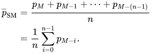
Moving Average Filter

In this technique, we average out the neighboring values along with the original cost. For example, for a MAF of 3, we add the current value, the value preceding the current value, the value succeeding the current value and divide it by three.

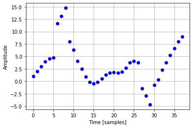
Let’s write the code for the above example and plot it after using MAF of 3 and 4 Respectively.

arr=[1,2,3,4,5,6,5,4,40,5,4,3,2,1,-1,-2,-1,0,1,2,3,2,1,2,3,5,6,3,2,-20,1,0,3,4,5,7,8,9]
length=len(arr)
#MAF of 3
for i in range(1,len(arr)-1):
    arr[i]=(arr[i-1]+arr[i]+arr[i+1])/3
plt.plot(np.arange(0,38), arr, 'ro')
plt.xlabel('Time [samples]')
plt.ylabel('Amplitude')
plt.grid(True)
plt.show()

#Moving Average(5) Filter
arr=[1,2,3,4,5,6,5,4,40,5,4,3,2,1,-1,-2,-1,0,1,2,3,2,1,2,3,5,6,3,2,-20,1,0,3,4,5,7,8,9]
length=len(arr)
for i in range(2,len(arr)-2):
    arr[i]=(arr[i-2]+arr[i-1]+arr[i]+arr[i+1]+arr[i+2])/5
plt.plot(np.arange(0,38), arr, 'bo')
plt.xlabel('Time [samples]')
plt.ylabel('Amplitude')
plt.grid(True)
plt.show()

#Moving Average(5) cascaded with another MAF 5 Filter
length=len(arr)
for i in range(2,len(arr)-2):
    arr[i]=(arr[i-2]+arr[i-1]+arr[i]+arr[i+1]+arr[i+2])/5
plt.plot(np.arange(0,38), arr, 'go')
plt.xlabel('Time [samples]')
plt.ylabel('Amplitude')
plt.grid(True)
plt.show()

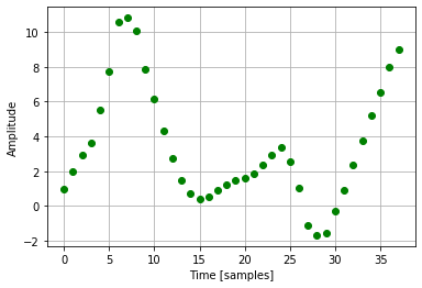
We have used equal weight for each component here. We can also proceed by unequal weights such that the points which far away have lower weight components compared to closer ones. This is known as Filtering with a weighted moving average.

One One thing we notice with any of the above mentioned MAF techniques is that the processed signal is, despite its increased smoothness, quite different from the original signal.

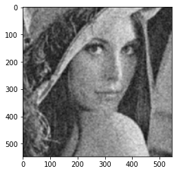
2D MAF with images

We take grid of dimension m by n and find the average value of all pixels in this grid. In this proWe take a grid of dimension m by n and find the average value of all pixels in this grid. In this process, we might lose the boundary of the image as an average around the pixel to be replaced is calculated. If m and n are both 5, we start with 3rd row, 3rd column, and calculate the average of 24 points(5*5 – the current pixel point) around this point.

#Vanilla Code
import cv2 as cv
import matplotlib
img = cv.imread('4.png')
cols=len(img[0])
rows=len(img)

#Grid Size 9 
m=9
n=9
gray = cv.cvtColor(img, cv.COLOR_BGR2GRAY)
grayarray=(np.array(gray))
newimage=[]
for i in range(0,rows-m):
    imagerow=[]
    for j in range(0,cols-n):
        sumofpixelvalues=0
        for i1 in range(0,m):
            for j1 in range(0,n):
                sumofpixelvalues=sumofpixelvalues+grayarray[i+i1][j+j1]
        average=sumofpixelvalues/(m*n)
        imagerow.append(int(average))
    newimage.append(imagerow)

newimage=np.array(newimage)
matplotlib.pyplot.imshow(newimage,cmap='gray', vmin=0, vmax=255)

That’s all for this post. Hope you liked it. In the next post we will discuss how the drawbacks of MAF i.e., distinctness of original and processed signals be reduced by Median Filter insted of Moving Average Filter. Leave any comments or suggestions below.

See you soon 🙂